Workflows for pangenomics
Since PanTools has many subcommands, we have created a number of workflows to help you get started.
Finding core, accessory and unique genes
One of the most common tasks for a pangenome analysis is to find the core,
accessory and unique genes in a set of genomes. For this, you needs to
calculate homology groups and then find the core, accessory and unique genes.
Homology grouping can be done using the group command if you already has
a set of parameters for the homology search. If not, the optimal_grouping
command can be used to find the optimal parameters for a given set of
proteins. This core, accessory and unique analysis can be performed for both
pangenomes and panproteomes.
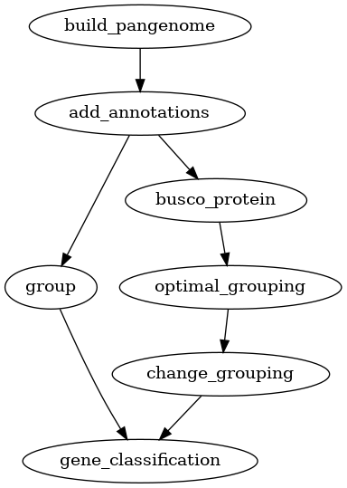
Fig. 2 Workflow for finding core, accessory and unique genes in a pangenome.
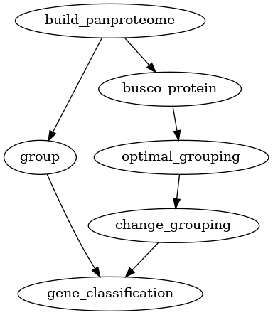
Fig. 3 Workflow for finding core, accessory and unique genes in a panproteome.
Creating phylogenetic trees
PanTools has six different commands for creating phylogenetic trees. However, some methods are specific to a pangenome since they work on nucleotide sequences. Optionally, you can also add phenotype information to the PanTools database and use this information to color the tree.
![digraph G {
"build_pangenome" -> "add_annotations";
"build_pangenome" -> "add_phenotype" [style=dashed];
"add_annotations" -> "group";
"add_annotations" -> "busco_protein";
"busco_protein" -> "optimal_grouping";
"optimal_grouping" -> "change_grouping";
"group" -> "gene_classification";
"change_grouping" -> "gene_classification";
"add_phenotype" -> "gene_classification" [style=dashed];
"gene_classification" -> "gene_distance_tree.R";
"add_phenotype" -> "kmer_classification" [style=dashed];
"build_pangenome" -> "kmer_classification";
"add_phenotype" -> "ani" [style=dashed];
"build_pangenome" -> "ani";
"kmer_classification" -> "genome_kmer_distance_tree.R";
"gene_classification" -> "core_phylogeny";
"gene_classification" -> "mlsa_find_genes";
"mlsa_find_genes" -> "mlsa_concatenate";
"mlsa_concatenate" -> "mlsa";
"gene_classification" -> "consensus_tree";
}](../_images/graphviz-8c71059176e5b958a774d27128807b9149bb95b2.png)
Fig. 4 Workflow for creating phylogenetic trees with a pangenome.
![digraph P {
"build_panproteome" -> "add_phenotype" [style=dashed];
"build_panproteome" -> "group";
"build_panproteome" -> "busco_protein";
"busco_protein" -> "optimal_grouping";
"optimal_grouping" -> "change_grouping";
"group" -> "gene_classification";
"change_grouping" -> "gene_classification";
"add_phenotype" -> "gene_classification" [style=dashed];
"gene_classification" -> "gene_distance_tree.R";
"add_phenotype" -> "ani" [style=dashed];
"build_panproteome" -> "ani";
"gene_classification" -> "core_phylogeny";
"gene_classification" -> "mlsa_find_genes";
"mlsa_find_genes" -> "mlsa_concatenate";
"mlsa_concatenate" -> "mlsa";
"gene_classification" -> "consensus_tree";
}](../_images/graphviz-e63775ff789c1466a1ccb00438f10b4a59fdaf15.png)
Fig. 5 Workflow for creating phylogenetic trees with a panproteome.
Mapping reads
PanTools has a map subcommand for mapping WGS reads to a pangenome. This
subcommand can be used to map reads to a pangenome only.
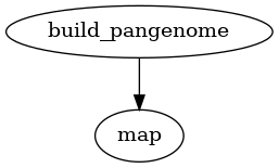
Fig. 6 Workflow for mapping reads to a pangenome.
Adding variants
Two types of variation can be added to a pangenome: VCF files and a PAV table.
VCF files can only be used for pangenomes, while PAV tables can be used for
both pangenomes and panproteomes. Creating homology groups is not needed for
adding these two types of variation but it is needed for the downstream
analyses. Alternatively to group as used in the graphs below, you can also
use the busco_protein, optimal_grouping and change_grouping chain
of commands.
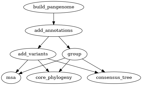
Fig. 7 Workflow for adding variants (VCF) to a pangenome.
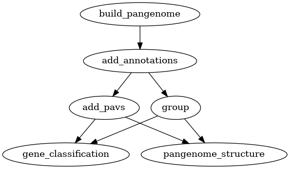
Fig. 8 Workflow for adding variants (PAV) to a pangenome.
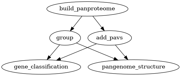
Fig. 9 Workflow for adding variants (PAV) to a panproteome.