Pangenome characterization
Functionalities for characterization a pangenome based on genes, k-mer sequences and functions. In this manual we use several pangenome related terms with the following definitions:
Core, an element is present in all genomes
Unique, an element is present in a single genome
Accessory, an element is present in some but not all genomes
When phenotype information is used in the analysis, three additional categories can be assigned:
Shared, an element present in all genomes of a phenotype
Exclusive, an element is only present in a certain phenotype
Specific, an element present in all genomes of a phenotype and is also exclusive
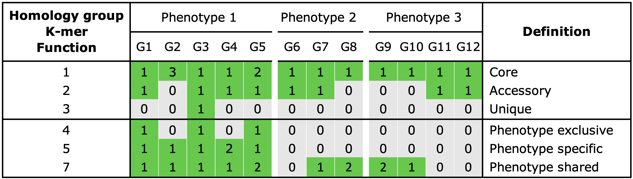
Fig. 3 The possible classification categories for genes, k mers and functions. Additional copies of an element are assigned to the same category.
Metrics
Generates relevant metrics of the pangenome and the individual genomes and sequences.
On the pangenome level: the number of genomes, sequences, annotations, genes, proteins, homology groups, k-mers, and database nodes and edges.
On the genome and sequence level: assembly statistics and metrics about functional elements. The assembly statistics consists of genome size, N25-N95, L25-L95, BUSCO scores and GC content. An overview of the functional elements is created by summarizing the functional annotations per genome (and sequence) and reporting the shortest, longest, average length and density per MB for genome features such as genes, exons and CDS.
Parameters
<databaseDirectory> |
Path to the database root directory. |
Options
|
Only include a selection of genomes. |
|
Exclude a selection of genomes. |
|
A text file with the identifiers of annotations that should be used. The most recent annotation is selected for genomes without an identifier. |
Example commands
$ pantools metrics tomato_DB
$ pantools metrics --exclude=1,2,5 tomato_DB
Output
Output files are written to the metrics directory in the database. Note: the percentage a genome or sequence is covered by a genes, repeats etc., (currently) does not consider overlap between features!
metrics.txt, overview of the metrics calculated on the pangenome and genome level.
metrics_per_genome.csv, summary of the metrics that are calculated on a genome level. The output is formatted as table.
metrics_per_sequence.csv, summary of metrics that are calculated on a sequence (contig/scaffold) level. The output is formatted as table. This file is not created when using a panproteome.
Homology groups
The following functions require the protein sequences to be clustered by group.
Gene classification
Classification of the pangenome’s gene repertoire. Homology groups are utilized to identify shared genes between genomes. The default criteria for defining the category of a gene is shown in Fig. 3.
To identify soft core and cloud genes, the core and unique thresholds (%)
can be relaxed by --core-threshold and --unique-threshold,
respectively. The --phenotype-threshold argument can be used to
lower the threshold for phenotype specific and shared homology groups.
Parameters
<databaseDirectory> |
Path to the database root directory. |
Options
|
Only include a selection of genomes. This automatically lowers the threshold for core genes. |
|
Exclude a selection of genomes. This automatically lowers the threshold for core genes. |
|
A phenotype name, used to find genes specific to the phenotype. |
|
Finds suitable single-copy groups for a MLSA. |
|
Threshold (%) for (soft) core genes. Default is 100% of genomes. |
|
Threshold (%) for unique/cloud genes. Default is a single genome, not a percentage. |
|
Threshold (%) for phenotype specific/shared genes. Default is 100% of genomes with phenotype. |
Example commands
$ pantools gene_classification tomato_DB
$ pantools gene_classification --unique-threshold=5 --core-threshold=95 tomato_DB
$ pantools gene_classification --phenotype=resistance --exclude=2,3 --phenotype-threshold=95 tomato_DB
Output
Output files are written to the gene_classification directory in the database.
gene_classification_overview.txt, statistics of the core, accessory, unique groups of the pangenome and individual genomes.
classified_groups.csv, the classified homology groups formatted as the table in the example table above.
cnv_core_accessory.txt, core and accessory groups with genomes that have additional copies compared to the lowest number (at least 1) in the group.
group_size_occurrence.txt, number of times a group of a certain size occurs in the pangenome. The homology group sizes can be based on the number of proteins or the number of genomes.
gene_distance_tree.R, an R script to cluster genomes based on gene distance (absence/presence). For more information, see the Gene distance tree manual.
shared_unshared_gene_count.csv, six tables with the number of shared and unshared genes between genomes: all genes, distinct genes and informative distinct genes. To get the number of distinct genes, additional copies of a gene within a homology group are ignored. Genes are considered informative when shared by at least two genomes.
Additional files are generated when the --phenotype argument is
included.
gene_classification_phenotype_overview.txt, the number of identified phenotype shared and specific groups.
phenotype_disrupted.txt, this file shows which proteins prevented phenotype shared groups to be specific.
phenotype_cnv, homology groups where all members of a phenotype have at least one additional copy of a gene compared to one of the other phenotypes.
phenotype_association.csv, results of performed Fisher exact tests on homology groups with an unequal proportion of phenotype members.
The following files contain homology group node identifiers.
all_homology_groups.csv, the node identifiers of all homology groups.
core_groups.csv, the node identifiers of the core homology groups.
single_copy_orthologs.csv, the node identifiers of single-copy ortholog groups. This is a subset of the core set where each genome is only allowed to have a one copy of a gene.
accessory_groups.csv, the node identifiers of accessory homology groups. The groups are ordered (in descending order) by the group size based on the total number of genomes present.
accessory_combinations.csv, the node identifiers of accessory homology groups, ordered by the combination of genomes by which they are shared.
unique_groups.csv, the node identifiers of unique homology groups ordered by genome.
phenotype_specific_groups.csv, the node identifiers of phenotype specific homology groups.
phenotype_shared_groups.csv, the node identifiers of phenotype shared homology groups.
phenotype_exclusive_groups.csv, the node identifiers of phenotype exclusive homology groups.
When --mlsa is included
mlsa_suggestions.txt, a list of single copy ortholog genes all having the same gene name. This file cannot be created when using a panproteome.
Core unique thresholds
Runs a simplified version of the gene_classification function to
test the effect of different --core-threshold and
--unique-threshold cut-offs between 1 and 100%.
Parameters
<databaseDirectory> |
Path to the pangenome database root directory. |
Options
|
Only include a selection of genomes. This automatically lowers the threshold for core genes. |
|
Exclude a selection of genomes. This automatically lowers the threshold for core genes. |
Example commands
$ pantools core_unique_thresholds tomato_DB
$ pantools core_unique_thresholds --exclude=1,2,5-10 tomato_DB
$ R script tomato_DB/R_scripts/core_unique_thresholds/core_unique_thresholds.R
Output
Output files are written to core_unique_thresholds directory in the database.
core_unique_thresholds.csv, the number of (soft) core unique/cloud homology groups for all tested thresholds.
core_unique_thresholds.R, the R script plots the number of (soft) core unique/cloud homology groups for all tested thresholds.
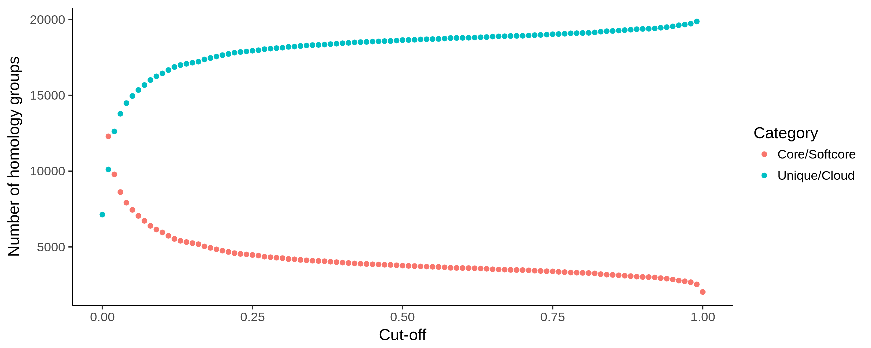
Fig. 4 Example output of core_unique_thresholds.R on a pangenome of 197 Pectobacterium genomes demonstrates the effect of loosening the thresholds. The number of (soft) core (orange) homology groups slightly increases when the cut-off for this category is lowered from 100% (200 genomes) to 1% (2) in steps of 1%. Unique/cloud (blue) start at 0.00 which represents a single genome. Using a 0.01 cut-off, groups are unique/cloud having 2 genomes or less. The threshold is further increased to 100% (200) in steps of 1%.
Grouping overview
Reports the content of all (active & inactive) homology groups for the
different groupings in the pangenome. Include --fast into the
command to get a quick overview of the available groupings and the
settings that were used.
Parameters
<databaseDirectory> |
Path to the pangenome database root directory. |
Options
|
Only show which grouping is active and which groupings can be activated. |
Example commands
$ pantools grouping_overview tomato_DB
$ pantools grouping_overview --fast tomato_DB
Output
Output files are written to /database_directory/group/
grouping_overview.txt, all homology groups in the pangenome. For each homology group, the total number of members and the number of members per per genome is reported.
current_pantools_homology_groups.txt, overview of the active homology groups. Each line represents one homology group. The line starts with the homology group (database) identifier followed by a colon and the rest are mRNA IDs (from gff/genbank) seperated by a space.
Pangenome structure
Iterations of random genome combinations according to the models proposed by Tettelin et al.* in 2005 are used to determine the contribution of new accessions with respect to the increase in core, accessory, and unique. Each iteration starts with three random genomes from which core, accessory and unique homology groups are identified. Subsequently, random genomes are added and group reclassified until the maximum number of genomes is reached. To simulate the overall pangenome-size increase and core-genome decrease, we suggest to use at least 10,000 iterations. Additional copies of a gene are ignored in the simulation.
Heaps’ law (a power law) can be fitted to the number of new genes observed when increasing the pangenome by one random genome. The formula for the power law model is \(n = k * N^{-a}\), where n is the newly discovered genes, N is the total number of genomes, and k and a are the fitting parameters. A pangenome can be considered open when a < 1 and closed if a > 1.
Pangenome size estimation is based on homology groups. This function
requires the sequences to be already clustered by
group. The same simulation can be performed
on k-mer sequences instead of homology groups with --kmer. As the number
of k-mers is significantly higher than the number of homology groups, the
runtime is much longer and the (default) number of loops is set to only 100.
Parameters
<databaseDirectory> |
Path to the pangenome database root directory. |
Options
|
Only include a selection of genomes. |
|
Only include a selection of genomes. |
|
Exclude a selection of genomes. |
|
Pangenome size estimation based on k-mer sequences (homology-groups is default). |
|
Number of loops (default is 10.000 for homology groups, 100 for k-mers). |
Example commands
$ pantools pangenome_structure tomato_DB
$ pantools pangenome_structure --loops=1000 --exclude=1-3,5  tomato_DB
$ pantools pangenome_structure --kmer tomato_db

$ R script pangenome_growth.R
$ R script gains_losses_median_or_average.R
$ R script gains_losses_median_and_average.R
$ R script heaps_law.R
$ R script core_access_unique.R
Output
Output files for homology-group based estimation are written to /database_directory/pangenome_size/gene/
pangenome_size.txt, various statistics on the number core, accessory, and unique homology groups for the different pangenome sizes.
gains_losses.txt, the average group gain and loss between different pangenome sizes. First the average number (core, accessory, and unique) groups for each pangenome size is calculated. The average gain and loss of groups is then found by subtracting the averages of a certain size to the averages of one genome larger (e.g. pangenome size of 5 is compared to 6).
gains_losses_last_genome.txt, the number of (core, accessory, and unique) groups that are gained or lost when including one of the genomes to a pangenome of the remaining genomes.
pangenome_growth.R, an R script to plot the number of core, accessory and unique groups for the different genome combinations. Second option is to only plot a core and accessory curve by including unique groups to the accessory.
gains_losses_median_and/or_average.R, R scripts to plot the average and median group gain and loss between pangenome sizes.
heaps_law.R, an R script to perform Heaps’ law.
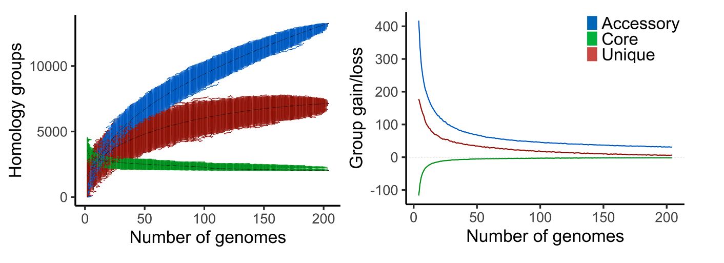
Fig. 5 Example output of pangenome_growth.R (left) and gains_losses_median_and_average.R (right) on a pangenome of 204 bacteria.
Output files for k-mer based estimation are written to /database_directory/pangenome_size/kmer/
pangenome_size_kmer.txt, statistics of the number of k-mers with different pangenome sizes.
core_access_unique.R, an R script to plot the number core, accessory, unique k-mers for the different genome combinations.
core_access.R, an R script to plot the number of core and accessory (including unique) k-mers for the different genome combinations.
Relevant literature
K-mer classification
Calculate the number of core, accessory, unique, (and phenotype
specific) k-mer sequences. Because k-mer sequences of non-branching
paths of the DBG graph are collapsed into a single node, k-mers are
first uncompressed before they are counted. When --compressed
is included, sequences are not uncompressed and considered as a single
k-mer. Nucleotide nodes with a ‘degenerate’ label contain letters
other than the four non-ambiguous ones (A, T, C, G). and are ignored by
this function.
Parameters
<databaseDirectory> |
Path to the pangenome database root directory. |
Options
|
Only include a selection of genomes. This automatically lowers the threshold for core k-mers. |
|
Exclude a selection of genomes. This automatically lowers the threshold for core k-mers. |
|
A phenotype name, used to identify phenotype specific k-mers. |
|
Do not uncompress collapsed non-branching k-mers for k-mer counting. |
|
Threshold (%) for (soft) core k-mers. Default is 100% of the genomes. |
|
Threshold (%) for unique/cloud k-mers. Default is a single genome, not a percentage. |
|
Threshold (%) for phenotype specific/shared k-mers. Default is 100% of genomes with phenotype. |
Example commands
$ pantools kmer_classification tomato_DB
$ pantools kmer_classification --phenotype=resistant --exclude=2,3,4 tomato_DB
$ pantools kmer_classification --compressed --core-threshold=95 --unique-threshold=5 tomato_DB
Output
Output files are written to /database_directory/kmer_classification/
kmer_classification_overview.txt, some general statistics and percentages about the core, accessory unique k-mers per genome.
kmer_occurrence.txt, the occurrence of k-mers per genome and total occurrence in the pangenome.
kmer_distance_tree.R, an R script to cluster genomes with four different k-mer distances to choose from. For more information, see The k-mers are ordered from high to low by the total number of genomes the k-mer is found.
unique_kmers.csv, the node identifiers of unique k-mers ordered by genome.
phenotype_specific_kmers.csv, the node identifiers of phenotype specific k-mers.
phenotype_shared_kmers.csv, the node identifiers of phenotype shared k-mers.
Functional annotations
The following functions can only be used when any type of functional annotation is added to the database.
Functional classification
Similar to gene and k-mer classification, this function identifies core, accessory, unique functional annotations in the pangenome. Only the following functions are considered for this analysis: biosynthetic gene clusters from antiSMASH, GO, PFAM, InterPro, TIGRFAM.
Parameters
<databaseDirectory> |
Path to the pangenome database root directory. |
Options
|
Only include a selection of genomes. This automatically lowers the threshold for core genes. |
|
Exclude a selection of genomes. This automatically lowers the threshold for core genes. |
|
A text file with the identifiers of annotations that should be used. The most recent annotation is selected for genomes without an identifier. |
|
A phenotype name, used to find functions specific to a phenotype. |
|
Threshold (%) For (soft) core functions (default is 100%). |
|
Threshold (%) For unique/cloud functions (default is a single genome, not a percentage). |
Example commands
$ pantools functional_classification tomato_DB
$ pantools functional_classification -p=flowering_time tomato_DB
Output
Output files are written to /database_directory/function/functional_classification/
functional_annotation_overview, number of core, accessory, and unique functions. Holds the number of phenotype shared and specific functions when a phenotype is included.
core_functions.txt, functional annotations found in every genome of the pangenome.
accessory_functions.txt, functional annotations labeled as accessory.
unique_functions.txt, functional annotations unique to a single genome.
When a --phenotype is included
phenotype_shared_functions.txt, functional annotations shared by all phenotype members.
phenotype_specific_functions.txt, functional annotations specific to certain phenotypes.
Function overview
Creates several summary files for each type of functional annotation present in the database: GO, PFAM, InterPro, TIGRFAM, COG, Phobius, and biosynthetic gene clusters from antiSMASH. In addition to the functions that must be added via add_functional_annotations, this function also requires proteins to be clustered by group.
Parameters
<databaseDirectory> |
Path to the pangenome database root directory. |
Options
|
Only include a selection of genomes. |
|
Exclude a selection of genomes. |
|
A text file with the identifiers of annotations that should be used. The most recent annotation is selected for genomes without an identifier. |
Example commands
$ pantools function_overview tomato_DB
$ pantools function_overview --include=2-4 tomato_DB
Output
Output files are written to function directory in the database. The overview CSV files are tables with on each row a function identifier with the frequency of per genome and.
functions_per_group_and_mrna.csv, overview of all homology groups and the associated functions.
function_counts_per_group.csv,
go_overview.csv, overview of the GO terms in the pangenome.
pfam_overview.csv, overview of the PFAM domains in the pangenome.
tigrfam_overview.csv, overview of the TIGRFAMs in the pangenome.
interpro_overview.csv, overview of the InterPro domains in the pangenome.
bgc_overview.csv, overview of the added biosynthetic gene clusters from antiSMASH in the pangenome.
phobius_signalp_overview.csv, overview of the included Phobius transmembrane topology and signal peptide predictions in the pangenome.
cog_overview.csv, overview of the functional COG categories in the pangenome.
cog_per_class.R, an R script to plot the distribution of COG categories over the core, accessory, unique homology groups.
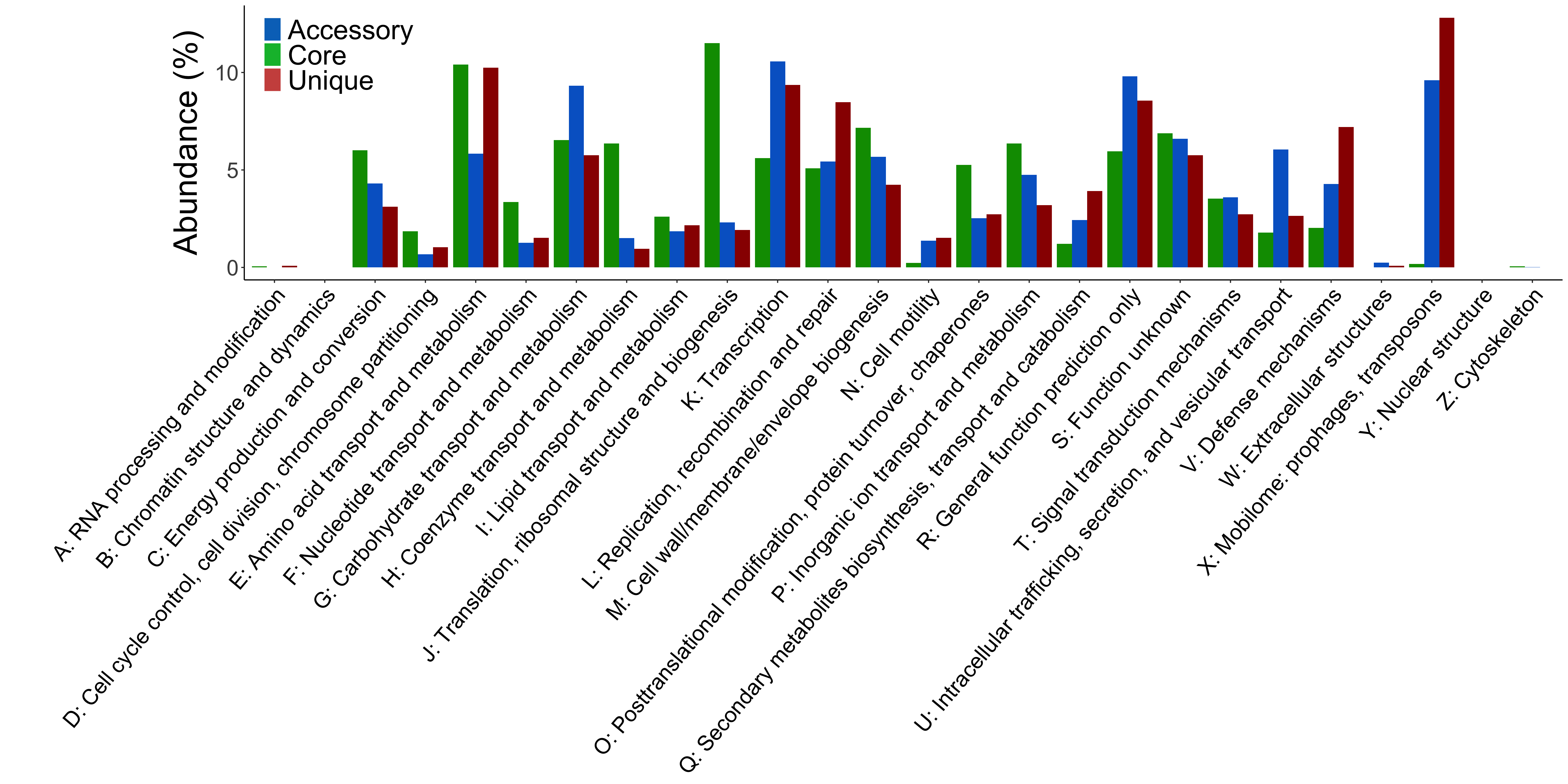
Fig. 6 Example output of cog_per_class.R. The proportion of COGs functional categories assigned to homology groups.
GO enrichment
For a given set of mRNA’s or homology groups, this function identifies over or underrepresented GO terms by using a hypergeometric distribution.
The p-value is calculated from the hypergeometric distribution
Parameter N = size of the population (Universe of genes).
Parameter n = size of the sample (signature gene set)
Parameter K = successes in population (enrichment gene set)
Parameter k = successes in sample (intersection of both gene sets)
Return the p-value of the Hypergeometric Distribution for P(X=k)
Prepare input for hypergeometric tests
The size and number of successes of the sample (n, k) and background (N, K) is prepared for each genome individually. Per genome, loops over every mRNA and checks for connected GO nodes. Each GO node connected to the mRNA is used to move up in the GO hierarchy via ‘is_a’ relations until the molecular_function, biological_process or cellular_component node is reached. Each GO term is counted only once per mRNA and a mRNA needs at least one GO term to be included in the sample and background sets. mRNA nodes which are part of the input homology groups are included into the sample set.
Multiple testing correction
Critical p-value using Bonferroni
For a GO germ to be significant, the p-value should be below 0.05 divided by number of tests per genome. For example, when 100 tests were performed, each p-value must be below 0.05/100 = 0.0005 to be considered significant.
Critical p-value using Benjamini-Hochberg procedure
Individual p-values are put in ascending order.
Ranks are assigned to the p-values. The lowest value has a rank of 1, the second lowest gets rank 2, etc..
The individual p-values Benjamini-Hochberg critical value is calculated using the formula \((i/m)Q\), where i is the individual p-values rank, m = total number of tests and Q is the false discovery rate.
Compare your original p-values to the critical B-H from Step 3; find the largest p value that is smaller than the critical value.
The critical p-value for the first rank for a total of 100 GO terms (tests) with a 5% false discovery rate is \((1/100) * 0.05 = 0.0005\). For the second and third rank this will be 0.0010 and 0.0015, respectively.
Required software
dot. Although this function still works when dot is not (properly) installed, no visualizations of the GO hierarchy can be created.
Parameters
<databaseDirectory> |
Path to the pangenome database root directory. |
Options
Requires one of --homology-file|--nodes.
|
A text file with homology group node identifiers, seperated by a comma. |
|
mRNA node identifiers, seperated by a comma on the command line. |
|
Only include a selection of genomes. |
|
Exclude a selection of genomes. |
|
The false discovery rate (percentage), default is 5%. |
Example commands
$ pantools go_enrichment -H=unique_groups.txt tomato_DB
$ pantools go_enrichment --fdr=1 -i=1-3,5 -H=pheno_specific.txt tomato_DB
Output
Output files are stored in /database_directory/function/go_enrichment/.
go_enrichment.csv, overview of all GO terms, p-values and the significance of enrichment. The output is formatted as a table.
go_enrichment_overview_per_go.txt, results of the analysis are ordered by GO term.
function_overview_per_mrna.txt, all functional annotations connected to the input sequences, ordered per mRNA.
function_overview_per_genome.txt, all functional annotations connected to the input sequences, ordered per genome.
Additional files are generated per individual genome and placed in /results_per_genome/.
go_enrichment.txt, list of GO terms, p-values and the critical p-values of Benjamin-Hochberg and Bonferroni.
revigo.txt, a list of GO terms and p-values that can be visualized on http://revigo.irb.hr
bio_process.pdf, dot visualisation of the Biological Process GO hierarchy.
cell_comp.pdf, dot visualisation of the Cellular Component GO hierarchy.
mol_function.pdf, dot visualisation of the Molecular Function GO hierarchy.
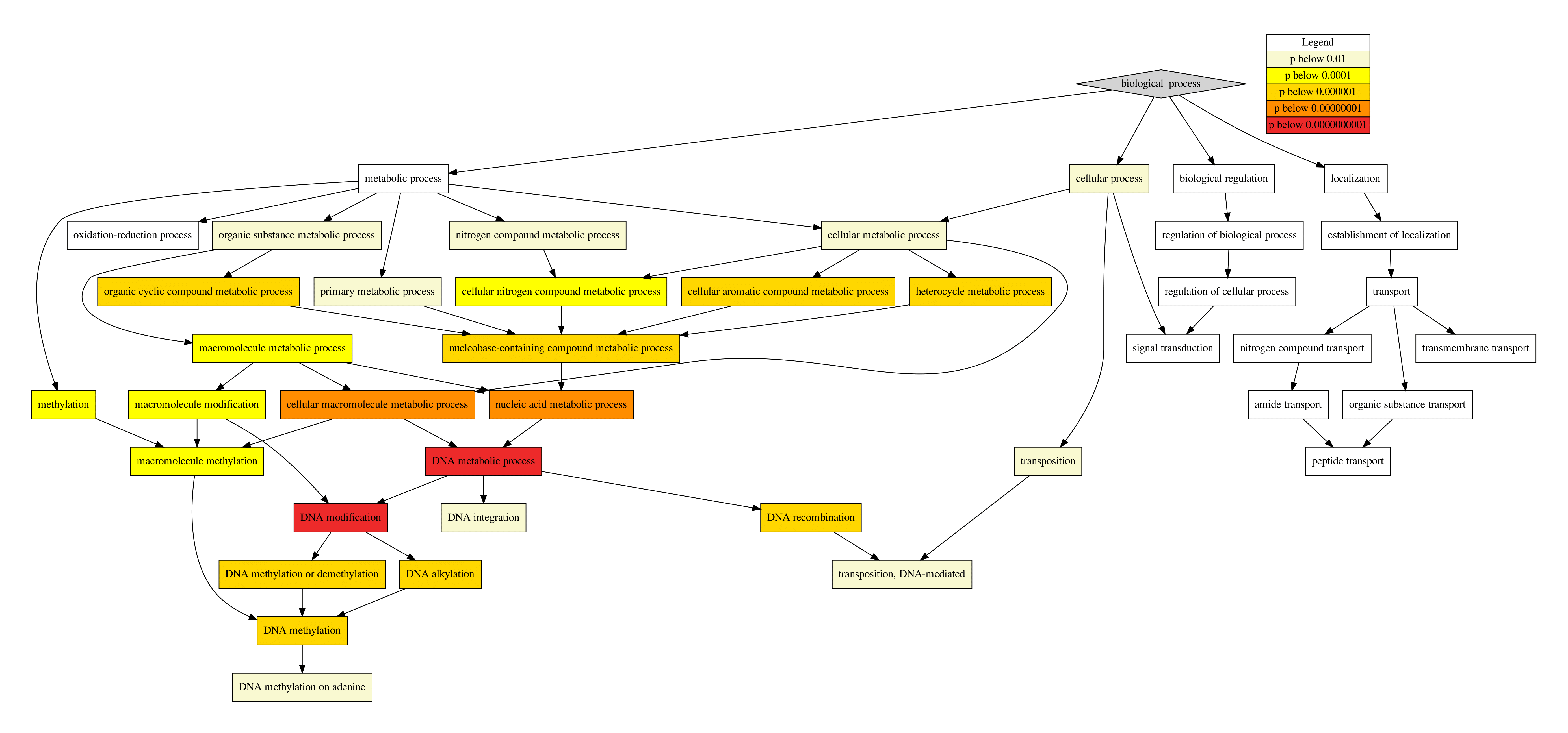
Fig. 7 Visualization of GO hierarchy by dot