Construct a pangenome

Build pangenome

Build a pangenome out of a set of genomes.

Required software

KMC 2.3 or 3.0

Parameters

<databaseDirectory>	Path to the database root directory.
<genomesFile>	A text file containing paths to FASTA files of genomes to be added to the pangenome; each on a separate line.

Options

--kmer-size

Size of k-mers. Should be in range [6..255]. By not giving this argument, the most optimal k-mer size is calculated automatically.

Example genomes file

/always/genome1.fasta
/use_the/genome2.fasta
/full_path/genome3.fasta

Example commands

$ pantools build_pangenome tomato_DB tomato_3.txt
$ pantools build_pangenome --kmer-size=15 tomato_DB tomato_3.txt

Relevant literature

• PanTools: representation, storage and exploration of pan-genomic data

---

Add annotations

Construct or expand the annotation layer of an existing pangenome. The layer consists of genomic features like genes, mRNAs, proteins, tRNAs etc. PanTools is only able to read General Feature Format (GFF) files.

Multiple annotations can be assigned to a single genome; however, only one annotation a time can be included in an analysis. The most recently included annotation of a genome is included as default, unless a different annotation is specified via --annotations-file, see the explanation below.

NB: GFF files are notoriously difficult to parse. PanTools uses htsjdk to parse GFF files, which is a Java library. Since we need to put this annotation in the graph database, it can be that the features are not correctly added. This is especially true for non-standard GFF files and annotated organellar genomes. If you encounter problems with a gff file, please check whether it is valid to the GFF3 specification. Also, our code should be able to handle all valid GFF3 files, but if the GFF3 file contains a trans-spliced gene that has alternative splicing, it will not be able to handle it (it will only annotate one mRNA).

Parameters

<databaseDirectory>	Path to the database root directory.
<annotationsFile>	A text file with on each line a genome number and the full path to the corresponding annotation file, separated by a space.

Options

--connect

Connect the annotated genomic features to nucleotide nodes in the DBG.

Example commands

$ pantools add_annotations tomato_DB annotations.txt
$ pantools add_annotations --connect tomato_DB annotations.txt

Output

The annotated features are incorporated in the graph. Output files are written to the database directory.

• annotation_overview.txt, a summary of the GFF files incorporated in the pangenome

• annotation.log, a list of misannotated feature identifiers.

Example input file

Each line of the file starts with the genome number followed by the full path to the annotation file. The genome numbers match the line number of the file that you used to construct the pangenome.

1 /always/genome1.gff
2 /use_the/genome2.gff
3 /full_path/genome3.gff

GFF3 file format

The GFF format consists of one line per feature, each containing 9 columns of data, plus optional track definition lines, that must be tab separated. Please use the proper hierarchy for the feature: gene -> mRNA -> CDS. Where gene is the parent of mRNA and mRNA is the parent of the CDS feature. The following example from Saccharomyces cerevisiae YJM320 (GCA_000975885) displays a correctly formatted gene entry:

CP004621.1      Genbank gene    44836   45753   .       -       .       ID=gene99;Name=RPL23A;end_range=45753,.;gbkey=Gene;gene=RPL23A;gene_biotype=protein_coding;locus_tag=H754_YJM320B00023;partial=true;start_range=.,44836
CP004621.1      Genbank mRNA    44836   45753   .       -       .       ID=rna99;Parent=gene99;gbkey=mRNA;gene=RPL23A;product=Rpl23ap
CP004621.1      Genbank exon    45712   45753   .       -       .       ID=id112;Parent=rna99;gbkey=mRNA;gene=RPL23A;product=Rpl23ap
CP004621.1      Genbank exon    44836   45207   .       -       .       ID=id113;Parent=rna99;gbkey=mRNA;gene=RPL23A;product=Rpl23ap
CP004621.1      Genbank CDS     45712   45753   .       -       0       ID=cds92;Parent=rna99;Dbxref=SGD:S000000183,NCBI_GP:AJQ01854.1;Name=AJQ01854.1;Note=corresponds to s288c YBL087C;gbkey=CDS;gene=RPL23A;product=Rpl23ap;protein_id=AJQ01854.1
CP004621.1      Genbank CDS     44836   45207   .       -       0       ID=cds92;Parent=rna99;Dbxref=SGD:S000000183,NCBI_GP:AJQ01854.1;Name=AJQ01854.1;Note=corresponds to s288c YBL087C;gbkey=CDS;gene=RPL23A;product=Rpl23ap;protein_id=AJQ01854.1

Select specific annotations for analysis

Only one annotation per genome is considered by any PanTools functionality. When multiple annotations are included, the last added annotation of a genome is automatically selected unless an --annotations-file is included specifying which annotations to use. This annotation file contains only annotation identifiers, each on a separate line. The most recent annotation is used for genomes where no annotation number is specified in the file. Below is an example where the third annotation of genome 1 is selected and the second annotation of genome 2 and 3.

1_3
2_2
3_2

---

Grouping proteins

Group

Generate homology groups based on similarity of protein sequences. The resulting homology groups connect similar sequences in the pangenome database. Homology groups contain not only orthologous pairs, but also pairs of homologs duplicated after the speciation of the two species, so-called in-paralogs. The sizes of the groups are controlled by the --relaxation parameter that can be set very strict or more lenient, depending on the evolutionary distance of the genomes. When you are unsure which relaxation setting is most suitable for your dataset, running the optimal_grouping functionality is recommended.

Be aware that not every sequence within a homology group has to be similar to the other sequences. For example, two non-similar protein sequences each have a high-similarity hit with the same protein sequence but align to a different region, one at the start and one near the end of the sequence.

When you want to run group another time but with different parameters, the currently active grouping must first either be moved or removed. This can be achieved with the move or remove grouping functions.

Method

Here, we explain a simplified version of the original algorithm, please take a look at our publication for an extensive explanation. First, potential similar sequences are identified by counting shared k-mer (protein) sequences. Similarity between the selected protein sequences is calculated through (local) Smith-Waterman alignments. When the (normalized) similarity score of two sequences is above a given threshold (controlled by --relaxation), the proteins are connected with each other in the similarity graph. Every similarity component is then passed to the MCL (Markov clustering) algorithm to be possibly broken into several homology groups.

Relaxation

The relaxation parameter is a combination of four sub-parameters: intersection rate, similarity threshold, mcl inflation and contrast. The values for these parameters for each relaxation setting can be seen in the table below. We strongly recommend using the --relaxation option to control the grouping, but advanced users still have the option to control the individual sub-parameters.

Relaxation	1	2	3	4	5	6	7	8
Intersection rate	0.08	0.07	0.06	0.05	0.04	0.03	0.02	0.01
Similarity threshold	95	85	75	65	55	45	35	25
Mcl inflation	10.8	9.6	8.4	7.2	6.0	4.8	3.6	2.4
Contrast	8	7	6	5	4	3	2	1

Required software

MCL

Parameters

<databaseDirectory>

Path to the database root directory.

Options

--threads/-t	Number of parallel working threads, default is the number of available cores or 8, whichever is lower.
--include/-i	Only include a selection of genomes.
--exclude/-e	Exclude a selection of genomes.
--annotations-file/-A	A text file with the identifiers of annotations to be included, each on a separate line. The most recent annotation is selected for genomes without an identifier.
--longest	Only cluster protein sequences of the longest transcript per gene.
--relaxation	The relaxation in homology calls. Should be in range [1-8], from strict to relaxed. This argument automatically sets the four remaining arguments stated below.
--intersection-rate	The fraction of k-mers that needs to be shared by two intersecting proteins. Should be in range [0.001,0.1].
--similarity-threshold	The minimum normalized similarity score of two proteins. Should be in range [1..99].
--mcl-inflation	The MCL inflation. Should be in range [1,19].
--contrast	The contrast factor. Should be in range [0,10].

Example commands

$ pantools group -t=12 -r=4 tomato_DB
$ pantools group --intersection-rate=0.05 --similarity-threshold=65  --mcl-inflation=7.2 --contrast=5 tomato_DB

Output

• pantools_homology_groups.txt, overview of the created homology groups. Each line represents one homology group, starting with the homology group (database) identifier followed by a colon (:) and mRNA identifiers (from GFF) that are separated by a space. To ensure all identifiers are unique in this file, the mRNA ids are extended by a hash symbol (#) and a genome number. The following line is example output of an homology group with two genes from genome 1 and 146:

14001754: DLACAPHP_00001_mRNA#1 OPJEMMMF_03822_mRNA#146

Relevant literature

• Efficient inference of homologs in large eukaryotic pan-proteomes

---

Optimal grouping

Finding the most suitable settings for group can be difficult and is always dependent on evolutionary distance of the genomes in the pangenome. This functionality runs group on all eight --relaxation settings, from strictest (d1) to the most relaxed (d8). To find the optimal setting, complete and non-duplicated BUSCO genes that are present in all genomes are used to validate each setting.

Method

A perfect clustering of the sequences would place each BUSCO in a separate homology group with one representative protein per genome. When BUSCO is run against the pangenome, the proteins corresponding to the BUSCO HMMs have been identified. For each BUSCO, the representative proteins are checked whether these are clustered into a single or multiple groups. These groups are searched to identify sequences other than the current BUSCO. The highest number of correctly clustered BUSCOs present in one group are true positives (tp). Any other gene clustered inside this group is considered a false positive (fp) The remaining BUSCO genes outside this best group are counted as false negative (fn). The summation of tps fps and fns are defined as TP, FP and FN, respectively. From these scores recall, precision and F-score measures are calculated as follows:

\[ \begin{align}\begin{aligned}Recall &= \frac{TP}{TP + FN}\\Precision &= \frac{TP}{TP + FP}\\F-score &= 2 \frac{Recall * Precision}{Recall + Precision}\end{aligned}\end{align} \]

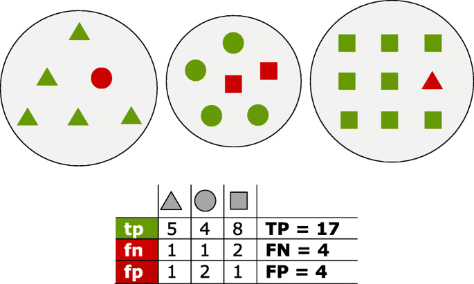
Fig. 1 Proteins of three distinct homology groups are represented as triangles, circles and squares. Green shapes are true positives (tp) which have been assigned to the true group; red shapes are false positives (fp) for the group they have been incorrectly assigned to, and false negatives (fn) for their true group

Choosing the optimal setting

Choosing the correct setting is usually a trade-off between TPs and FNs. The most strict grouping results in a significantly higher number of clusters as the more relaxed settings. With stringent settings, related proteins could get separated; however, a high number of false positives is (usually) prevented (FN > FP). When you would go for a more loose setting, the related proteins are likely to part of the same group, but other sequences could be included as well (FN < FP).

No grouping is active after running this function. Use the generated output files to identify a suitable grouping. Activate this grouping using change_grouping. An overview of the available groupings and used settings is stored in the ‘pangenome’ node (inside the database), or can be created by running grouping_overview.

Required software

MCL

Parameters

<databaseDirectory>	Path to the database root directory.
<buscoDirectory>	The output directory created by the busco_protein function. This directory is found inside the pangenome database, in the busco directory.

Options

--threads/-t	Number of parallel working threads, default is the number of available cores or 8, whichever is lower.
--include/-i	Only include a selection of genomes.
--exclude/-e	Exclude a selection of genomes.
--annotations-file/-A	A text file with the identifiers of annotations to be included, each on a separate line. The most recent annotation is selected for genomes without an identifier.
--fast	Assume the optimal grouping is found when the F1-score drops compared to the previous clustering round.
--longest	Only cluster protein sequences of the longest transcript per gene.
--relaxation	Only consider a selection of relaxation settings (1-8 allowed).

Example commands

$ pantools optimal_grouping bacteria_DB bacteria_DB/busco/bacteria_odb9
$ pantools optimal_grouping -t=12 --fast bacteria_DB bacteria_DB/busco/bacteria_odb9
$ pantools optimal_grouping -tn=12 --relaxation=1,2,3 bacteria_DB bacteria_DB/busco/bacteria_odb9

$ Rscript optimal_grouping.R

Output

After each clustering round, homology groups are incorporated in the graph. A text file with homology group and gene identifiers is stored in the group directory in the pangenome database. This file is named after the used sequence similarity threshold (25-95). Each line represents one homology group, starting with the homology group (database) identifier followed by a colon (:) and mRNA identifiers (from GFF) that are separated by a space. The mRNA identifiers are extended by a hash (#) and their genome number. The following line is example output of an homology group with two genes from genome 1 and 146:

14001754: DLACAPHP_00001_mRNA#1 OPJEMMMF_03822_mRNA#146

Output files are written to optimal_grouping directory inside the database.

• grouping_overview.csv, a summary of the benchmark statistics. Use this file to find the most suitable grouping for your pangenome.

• optimal_grouping.R, Rscript to plot FN and FP values per grouping.

• counts_per_busco.info, a log file of the scoring. Shows in which homology groups the BUSCO genes were placed for the different groupings.

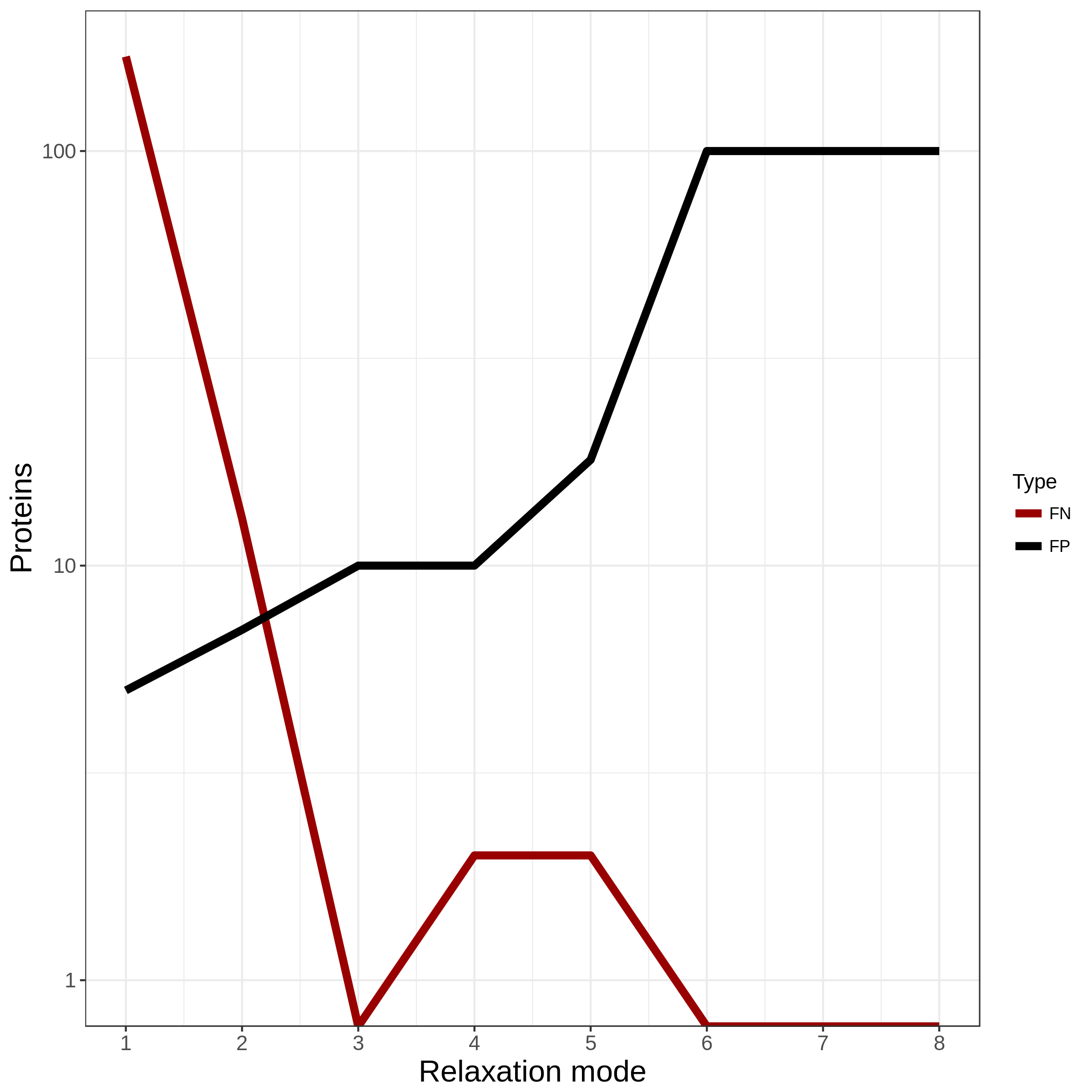
Fig. 2 Example output of optimal_grouping.R. The number of FN and FP for all eight relaxation settings.

---

Change grouping

Only a single homology grouping can be active in the pangenome. Use this function to change the active grouping version. Information of the available groupings and used settings is stored in the ‘pangenome’ node (inside the database) and can be created by running grouping_overview.

Parameters

<databaseDirectory>

Path to the database root directory.

Options

--grouping-version/-v

Required. The version of homology grouping to become active.

Example commands

$ pantools change_grouping -v=5 tomato_DB

---

Build panproteome

Build a panproteome out of a set of proteins. By only including protein sequences, the usable functionalities are limited to a protein-based analysis, please see differences pangenome and panproteome. No additional proteins can be added to the panproteome, it needs to be rebuilt completely.

Parameters

<databaseDirectory>	Path to the database root directory.
<proteomesFile>	A text file containing paths to FASTA files of proteins to be added to the panproteome; each on a separate line.

Example proteomes file

/always/proteins1.fasta
/use_the/proteins2.fasta
/full_path/proteins3.faa

Example commands

$ pantools build_panproteome proteome_DB proteins.txt

---

Add genomes

Add additional genomes to an existing pangenome.

Required software

KMC 2.3 or 3.0

Parameters

<databaseDirectory>	Path to the database root directory.
<genomesFile>	A text file containing paths to FASTA files of genomes to be added to the pangenome; each on a separate line.

Example genomes file

/use_the/genome4.fasta
/full_path/genome5.fasta

Example commands

$ pantools add_genomes pangenome_DB extra_genomes.txt

---

Add phenotypes

Including phenotype data to the pangenome which allows the identification of phenotype specific genes, SNPs, functions, etc.. Altering the data is done by rerunning the command with an updated CSV file.

Data types

Each phenotype node contains a genome number and can hold the following data types: String, Integer, Float or Boolean.

• Values recognized as round number are converted to an Integer and to a Double when having one or multiple decimals.

• Boolean types are identified by checking if the value matches ‘true’ or ‘false’, ignoring capitalization of letters.

• String values remain completely unaltered except for spaces and quotes characters. Spaces are changed into an underscore (’_’) character and quotes are completely removed.

Bin numerical values

When using numerical values, two genomes are only considered to share a phenotype if the value is identical. PanTools creates an alternative version for these phenotypes by binning the values. Taking ‘Pathogenicity’ from the example below we see the integers between 3 and 15. Using these two extreme values three bins are created for a new phenotype ‘Pathogenicity_binned’: 3-6.33, 6.34-11.66 and 11.67-15. The number of bins is controlled through --bins. For skewed data, consider making the bins manually and include this as string phenotype.

Parameters

<databaseDirectory>	Path to the database root directory.
<phenotypesFile>	A CSV file containing the phenotype information.

Options

--append	Do not remove existing phenotype nodes but only add new properties to them. If a property already exists, values from the new file will overwrite the old.
--bins	Number of bins used to group numerical values of a phenotype (default: 3).

Example phenotypes file

The input file needs to be in .CSV format, a plain text file where each value is separated by a comma. The first row should start with ‘Genome,’ followed by the phenotype names and/or identifiers. The first column must start with genome numbers corresponding to the one in your pangenome. Phenotypes and metadata must be placed on the same line as their genome number. A field can remain empty when the phenotype for a genome is missing or unknown. Here below is an example of five genomes contains six phenotypes:

Genome,Gram,Region,Pathogenicity,Boolean,float,species
1,+,NL,3,True,0.1,Species
2,+,BE,,False,0.1,Species3
3,+,LUX,7,true,0.1,Species3
4,+,NL,9,false,0.1,Species3
5,+,BE,15,TRUE,0.1,Species1

Example command

$ pantools add_phenotypes tomato_DB pheno.csv
$ pantools add_phenotypes --append tomato_DB pheno.csv

Output

Phenotype information is stored in ‘phenotype’ nodes in the graph. An output file is written to the database directory.

• phenotype_overview.txt, a summary of the available phenotypes in the pangenome

---

BUSCO protein

BUSCO attempts to provide a quantitative assessment of the completeness in terms of expected gene content of a genome assembly. Proteins are placed into categories of Complete and single-copy (S), Complete and duplicated (D), fragmented (F), or missing (M). This function is able to run BUSCO v3, v4 or v5 against protein sequences of the pangenome.

The number of reported duplicated genes in eukaryotes is often to high as different protein isoforms are counted multiple times. To adjust the imprecise duplication score, include the --longest-transcripts argument to the command.

You don’t have a benchmark set?

• When using BUSCO v3, go to https://busco.ezlab.org, download a odb9 set, and untar it with tar -xvzf. Include the entire directory in the command using the --input-file argument.

• For BUSCO v4 and v5, you only have to provide the odb10 database name with the --input-file argument, the database is downloaded automatically. To get a full list of the available datasets, run busco --list-datasets.

Required software

BUSCO must be set to your $PATH. For v3, test if the which run_BUSCO.py command displays the full path so it can accessed anywhere. For v4 and v5, test if busco is executable.

Parameters

<databaseDirectory>

Path to the database root directory.

Options

Requires one of --busco9|--busco10.

--threads/-t	Number of parallel working threads, default is the number of available cores or 8, whichever is lower.
--include/-i	Only include a selection of genomes.
--exclude/-e	Exclude a selection of genomes.
--annotations-file/-A	A text file with the identifiers of annotations to be included, each on a separate line. The most recent annotation is selected for genomes without an identifier.
--busco-version/-v	The BUSCO version. Select either ‘busco3’, ‘busco4’ or ‘busco5’ (default).
--busco9	An odb9 benchmark dataset file.
--busco10	An odb10 benchmark dataset name.
--longest	Only search against the longest protein-coding transcript of genes.
skip-busco	A list of questionable BUSCOs. The completeness score is recalculated by skipping these genes.

Example commands

$ pantools busco_protein --busco10=bacteria_odb10 bacteria_DB
$ pantools busco_protein -v=busco3 --busco9=busco_sets/bacteria_odb9/ bacteria_DB
$ pantools busco_protein --busco9=busco_sets/bacteria_odb9/ --skip-busco=POG093P01OY,POG093P0009,POG093P022K,POG093P027M,POG093P00Z2,POG093P013J bacteria_DB

Output

The BUSCO scores are stored inside BUSCO nodes of the pangenome graph. Output files are written to the busco directory inside the database.

• busco_scores.txt, overview of the BUSCO scores per genome. Average and median statistics are calculated per category.

• busco_overview.csv, a table which combines the completeness scores per genome together with the duplicated, fragmented and missing BUSCO genes.

• hmm_overview.txt, a list of BUSCO genes showing the assigned categories per genome.

---

Add functional annotations

PanTools is able to incorporate functional annotations into the pangenome by reading output from various functional annotation tools.

Add functions

This function can integrate different functional annotations from a variety of annotation files. Currently available functional annotations: Gene Ontology, Pfam, InterPro, TIGRFAM, Phobius, SignalP and COG. The first time this function is executed, the Pfam, TIRGRAM, GO, and InterPro databases are integrated into the pangenome. Phobius, SignalP and COG annotations do not have separate nodes and are directly annotated on ‘mRNA’ nodes in the pangenome.

Gene names (or identifiers) from the input file are used to identify gene nodes in the pangenome. Only genes with an exactly matching name/identifier can be connected to functional annotation nodes! Use the same FASTA and GFF3 files that were used to construct the pangenome database.

Functional databases

Database versions in PanTools repository

	Version	Download date (dd-mm-yyyy)
Gene ontology	2021-12-15	20-12-2021
Pfam	35.0	20-12-2021
TIGRFAM	15.0	01-10-2020
InterPro	87+	Not included in repository

We regularly check and update the four functional database. To update the functional database manually, download the following files and replace the old ones in the /pantools/addons/ directory. The TIGRFAM.info files are bundled in the TIGRFAMs_15.0_INFO.tar.gz file; download the file to addons/tigrfam and uncompress the tarball first. The first time running this function .INFO files are combined into a new file COMBINATION_INFO_FILES and removed afterwards.

File	Database type	Required directory	Download link
go.basic.obo	GO	addons	http://purl.obolibrary.org/obo/go/go-basic.obo
gene_ontology.txt	Pfam	addons	ftp://ftp.ebi.ac.uk/pub/databases/Pfam/releases//Pfam35.0/database_files/gene_ontology.txt.gz
Pfam-A.clans.tsv	Pfam	addons	ftp://ftp.ebi.ac.uk/pub/databases/Pfam/releases//Pfam35.0/Pfam-A.clans.tsv.gz
interpro.xml	InterPro	addons	https://ftp.ebi.ac.uk/pub/databases/interpro/current_release/interpro.xml.gz
TIGRFAMS_GO_LINK	TIGRFAM	addons/tigrfam	https://ftp.ncbi.nlm.nih.gov/hmm/TIGRFAMs/release_15.0/TIGRFAMS_GO_LINK
TIGRFAMS_ROLE_LINK	TIGRFAM	addons/tigrfam	https://ftp.ncbi.nlm.nih.gov/hmm/TIGRFAMs/release_15.0/TIGRFAMS_ROLE_LINK
TIGR_ROLE_NAMES	TIGRFAM	addons/tigrfam	https://ftp.ncbi.nlm.nih.gov/hmm/TIGRFAMs/release_15.0/TIGR_ROLE_NAMES
TIGR00001.INFO to TIGR04571.INFO	TIGRFAM	addons/tigrfam	https://ftp.ncbi.nlm.nih.gov/hmm/TIGRFAMs/release_15.0/TIGRFAMs_15.0_INFO.tar.gz

Parameters

<databaseDirectory>	Path to the database root directory.
<functionsFile>	A text file with on each line a genome number and the full path to the corresponding annotation file, separated by a space.

Options

`--annotations-file/-A

A text file with the identifiers of annotations to be included, each on a separate line. The most recent annotation is selected for genomes without an identifier.

Example commands

$ pantools add_functions tomato_DB f_annotations.txt
$ pantools add_functions -A annotations.txt tomato_DB f_annotations.txt

Output

Functional annotations are incorporated in the graph. A log file is written to the log directory.

• add_functional_annotations.log, a log file with the the number of added functions per type and the identifiers of functions that could not be included.

Example function files

The <functionsFile> requires to be formatted like an annotation input file. Each line of the file starts with the genome number followed by the full path to an annotation file.

File type	Recognized by pattern in file name
InterProScan	interpro & .gff
eggNOG-mapper	eggnog
Phobius	phobius
SignalP	signalp
Custom file	custom

1 /mnt/scratch/interpro_results_genome_1.gff
1 /mnt/scratch/custom_annotation_1.txt
1 /mnt/scratch/phobius_1.txt
2 /mnt/scratch/signalp.txt
2 /mnt/scratch/eggnog_genome_2.annotations
2 /mnt/scratch/transmembrane_annotations.txt phobius
3 /mnt/scratch/ipro_results_genome_3.annot custom

Annotation file types

PanTools can recognize functional annotations in different output formats.

Phobius and SignalP are not standard analyses of the InterProScan pipeline and require some additional steps during the InterProScan installation. Please take a look at our InterProScan install instruction to verify if the tools are part of the prediction pipeline. Phobius 1.01

Function type	Allowed annotation file
GO	InterProscan .gff & custom annotation file
Pfam	InterProscan .gff & custom annotation file
InterPro	InterProscan .gff & custom annotation file
TIGRFAM	InterProscan .gff & custom annotation file
Phobius	InterProscan .gff & Phobius 1.01 output
SignalP	InterProscan .gff, signalP 4.1 output, signalP 5.0 output
COG	eggNOG-mapper

InterProScan gff file:

##gff-version 3
##interproscan-version 5.52-86.0
AT4G21230.1   ProSiteProfiles protein_match 333 620 39.000664   +   .   date=06-10-2021;Target=mRNA.AT4G21230.1 333 620;Ontology_term="GO:0004672","GO:0005524","GO:0006468";ID=match$42_333_620;signature_desc=Protein kinase domain profile.;Name=PS50011;status=T;Dbxref="InterPro:IPR000719"
AT3G08980.5   TIGRFAM protein_match         25  101 3.7E-14     +   .   date=06-10-2021;Target=mRNA.AT3G08980.5 25 101;Ontology_term="GO:0006508","GO:0008236","GO:0016020";ID=match$66_25_101;signature_desc=sigpep_I_bact: signal peptidase I;Name=TIGR02227;status=T;Dbxref="InterPro:IPR000223"
AT2G17780.2   Phobius protein_match         338 354 .           +   .   date=06-10-2021;Target=AT2G17780.2 338 354;ID=match$141_338_354;signature_desc=Region of a membrane-bound protein predicted to be embedded in the membrane.;Name=TRANSMEMBRANE;status=T
AT2G17780.2   Phobius protein_match         1   337 .           +   .   date=06-10-2021;Target=AT2G17780.2 1 337;ID=match$142_1_337;signature_desc=Region of a membrane-bound protein predicted to be outside the membrane, in the extracellular region.;Name=NON_CYTOPLASMIC_DOMAIN;status=T
AT3G11780.2   SignalP_EUK protein_match     1   24  .           +   .   date=06-10-2021;Target=mRNA.AT3G11780.2 1 24;ID=match$230_1_24;Name=SignalP-noTM;status=T
AT1G04300.2   CDD protein_match             40  114 1.54717E-13 +   .   date=06-10-2021;Target=mRNA.AT1G04300.2 40 114;Ontology_term="GO:0005515";ID=match$212_40_114;signature_desc=MATH;Name=cd00121;status=T;Dbxref="InterPro:IPR002083"

eggNOG-mapper (tab separated) file:

#query_name     seed_eggNOG_ortholog seed_ortholog_evalue seed_ortholog_score best_tax_level Preferred_name GOs EC KEGG_ko KEGG_Pathway KEGG_Module KEGG_Reaction KEGG_rclass BRITE KEGG_TC CAZy BiGG_Reaction taxonomic scope eggNOG OGs best eggNOG OG COG Functional cat. eggNOG free text desc.
ATKYO-2G54530.1 3702.AT2G35130.2     1.9e-179             636.0               Brassicales     GO:0003674,GO:0003676,GO:0003723,GO:0003824,GO:0004518,GO:0004519,GO:0005488,GO:0005575,GO:0005622,GO:0005623,GO:0006139,GO:0006725,GO:0006807,GO:0008150,GO:0008152,GO:0009451,GO:0009987,GO:0016070,GO:0016787,GO:0016788,GO:0034641,GO:0043170,GO:0043226,GO:0043227,GO:0043229,GO:0043231,GO:0043412,GO:0044237,GO:0044238,GO:0044424,GO:0044464,GO:0046483,GO:0071704,GO:0090304,GO:0090305,GO:0097159,GO:1901360,GO:1901363                                           Viridiplantae   37R67@33090,3GAUT@35493,3HNDD@3699,KOG4197@1,KOG4197@2759   NA|NA|NA    E   Pentacotripeptide-repeat region of PRORP
ATKYO-UG22500.1 3712.Bo02269s010.1   7.5e-35              153.7               Brassicales                                                 Viridiplantae   29I9W@1,2RRH4@2759,383W6@33090,3GWQZ@35493,3I1A9@3699   NA|NA|NA
ATKYO-1G60060.1 3702.AT1G48090.1     0.0                  6241.0              Brassicales             ko:K19525                   ko00000             Viridiplantae   37IJB@33090,3GAN0@35493,3HQ90@3699,COG5043@1,KOG1809@2759   NA|NA|NA    U   Vacuolar protein sorting-associated protein
ATKYO-3G74720.1 3702.AT3G52120.1     7.2e-245             852.8               Brassicales             ko:K13096                   ko00000,ko03041             Viridiplantae   37QYY@33090,3G9VU@35493,3HRDK@3699,KOG0965@1,KOG0965@2759   NA|NA|NA    L   SWAP (Suppressor-of-White-APricot) surp domain-containing protein D111 G-patch domain-containing protein
ATKYO-4G41660.1 3702.AT4G16340.1     0.0                  3392.1              Brassicales     GO:0003674,GO:0005085,GO:0005088,GO:0005089,GO:0005488,GO:0005515,GO:0005575,GO:0005622,GO:0005623,GO:0005634,GO:0005737,GO:0005783,GO:0005829,GO:0005886,GO:0006810,GO:0008064,GO:0008150,GO:0008360,GO:0009605,GO:0009606,GO:0009628,GO:0009629,GO:0009630,GO:0009958,GO:0009966,GO:0009987,GO:0010646,GO:0010928,GO:0012505,GO:0016020,GO:0016043,GO:0016192,GO:0017016,GO:0017048,GO:0019898,GO:0019899,GO:0022603,GO:0022604,GO:0023051,GO:0030832,GO:0031267,GO:0032535,GO:0032956,GO:0032970,GO:0033043,GO:0043226,GO:0043227,GO:0043229,GO:0043231,GO:0044422,GO:0044424,GO:0044425,GO:0044432,GO:0044444,GO:0044446,GO:0044464,GO:0048583,GO:0050789,GO:0050793,GO:0050794,GO:0050896,GO:0051020,GO:0051128,GO:0051179,GO:0051234,GO:0051493,GO:0065007,GO:0065008,GO:0065009,GO:0070971,GO:0071840,GO:0071944,GO:0090066,GO:0098772,GO:0110053,GO:1902903     ko:K21852                   ko00000,ko04131             Viridiplantae   37QIM@33090,3G8RK@35493,3HSFN@3699,KOG1997@1,KOG1997@2759   NA|NA|NA    T   Belongs to the DOCK family

A custom input file must consist of two tab or comma separated columns. The first column should contain a gene/mRNA id, the second an identifier from one of four functional annotation databases: GO, Pfam, InterPro or TIGRFAM.

AT5G23090.4,GO:0046982
AT5G23090.4,IPR009072
AT1G27540.2,PF03478
AT2G18450.1,TIGR01816

Phobius 1.01 ‘short’ (tab separated) functions file:

SEQENCE ID                     TM SP PREDICTION
mRNA-YPR204W                    0  0 o
mRNA-ndhB-2_1                   6  Y n5-16c21/22o37-57i64-83o89-113i134-156o168-189i223-246o

Phobius 1.01 ‘long’ (tab separated) functions file:

ID   mRNA-YPR204W
FT   DOMAIN        1   1032       NON CYTOPLASMIC.
//
ID   mRNA-ndhB-2_1
FT   SIGNAL        1     21
FT   DOMAIN        1      4       N-REGION.
FT   DOMAIN        5     16       H-REGION.
FT   DOMAIN       17     21       C-REGION.
FT   DOMAIN       22     36       NON CYTOPLASMIC.
FT   TRANSMEM     37     57
FT   DOMAIN       58     63       CYTOPLASMIC.
FT   TRANSMEM     64     83
FT   DOMAIN       84     88       NON CYTOPLASMIC.
FT   TRANSMEM     89    113
FT   DOMAIN      114    133       CYTOPLASMIC.
FT   TRANSMEM    134    156
FT   DOMAIN      157    167       NON CYTOPLASMIC.
FT   TRANSMEM    168    189
FT   DOMAIN      190    222       CYTOPLASMIC.
FT   TRANSMEM    223    246
FT   DOMAIN      247    253       NON CYTOPLASMIC.
//

SignalP 4.1 ‘short’ (tab separated) functions file:

# name                     Cmax  pos  Ymax  pos  Smax  pos  Smean   D     ?  Dmaxcut    Networks-used
mRNA-rpl2-3                0.148  20  0.136  20  0.146   3  0.126   0.131 N  0.450      SignalP-noTM
mRNA-cox2                  0.107  25  0.132  12  0.270   4  0.162   0.148 N  0.450      SignalP-noTM
mRNA-cox2_1                0.850  17  0.776  17  0.785   2  0.717   0.753 Y  0.500      SignalP-TM

SignalP 5.0 ‘short’ (tab separated) functions file:

# SignalP-5.0 Organism:   Eukarya     Timestamp: 20211122233246
# ID          Prediction  SP(Sec/SPI) OTHER    CS Position
AT3G26880.1   SP(Sec/SPI) 0.998803    0.001197 CS pos: 21-22. VYG-KK. Pr: 0.9807
mRNA-rpl2-3   OTHER       0.001227    0.998773

Relevant literature

• Expansion of the Gene Ontology knowledgebase and resources

• InterPro in 2019: improving coverage, classification and access to protein sequence annotations

• TIGRFAMs and Genome Properties in 2013

• A Combined Transmembrane Topology and Signal Peptide Prediction Method

• Expanded microbial genome coverage and improved protein family annotation in the COG database

---

Add antiSMASH

Read antiSMASH output and incorporate Biosynthetic Gene Clusters (BGC) nodes into the pangenome database. A ‘bgc’ node holds the gene cluster product, the cluster address and has a relationship to all gene nodes of the cluster. For this function to work, antiSMASH should be performed with the same FASTA and GFF3 files used for building the pangenome. antiSMASH output will not match the identifiers of the pangenome when no GFF file was included.

As of PanTools v3.3.4 the required antiSMASH version is 6.0.0. Gene cluster information is parsed from the .JSON file that is generated in each run. We try to keep the parser updated with newer versions but please contact us when this is no longer the case.

	Version	Version Date
antiSMASH	6.0.0	21-02-2021

Parameters

<databaseDirectory>	Path to the database root directory.
<antiSMASHFile>	A text file with on each line a genome number and the full path to the corresponding antiSMASH output file, separated by a space.

Options

--annotations-file/-A

A text file with the identifiers of annotations to be included, each on a separate line. The most recent annotation is selected for genomes without an identifier.

Example antiSMASH file

The <antiSMASHFile> requires to be formatted like a regular annotation input file. Each line of the file starts with the genome number followed by the full path to the JSON file.

1 /mnt/scratch/IPO3844/antismash/IPO3844.json
4 /home/user/IPO3845/antismash/IPO3845.json

Example commands

$ pantools add_antismash tomato_DB clusters.txt
$ pantools add_antismash -A annotations.txt tomato_DB clusters.txt

---

Removing data

The following functionalities allow the removal of large sets of nodes and relationships from the pangenome. These functions will first ask for a confirmation before the nodes are actually removed. Be careful, the data is not backed up and removing nodes or properties means it is permanently gone.

---

Remove nodes

Remove a selection of nodes and their relationships from the pangenome. For a pangenome database the following nodes should never be removed: nucleotide, pangenome, genome, sequence. When using a panproteome, mRNA nodes cannot be removed.

Parameters

<databaseDirectory>

Path to the database root directory.

Options

Requires one of --nodes|--label, include and exclude only work for --label.

--include/-i	Only remove nodes of the selected genomes.
--exclude/-e	Do not remove nodes of the selected genomes.
--nodes/-n	One or multiple node identifiers, separated by a comma.
--label	A node label, all nodes matching the label are removed.

Example commands

$ pantools remove_nodes --nodes=10348734,10348735,10348736 tomato_DB
$ pantools remove_nodes --label=busco --include=2-6 tomato_DB

---

Remove phenotypes

Delete phenotype nodes or remove specific phenotype information from the nodes. The specific phenotype property needs to be specified with --phenotype. When this argument is not included, phenotype nodes are removed.

Parameters

<databaseDirectory>

Path to the database root directory.

Options

--include/-i	Only remove nodes of the selected genomes.
--exclude/-e	Do not remove nodes of the selected genomes.
--phenotype/-p	Name of the phenotype. All information of the given phenotype is removed from ‘phenotype’ nodes.

Example commands

$ pantools remove_phenotype tomato_DB
$ pantools remove_phenotype --phenotype=color tomato_DB
$ pantools remove_phenotype --phenotype=color --exclude=11,12 tomato_DB

---

Remove annotations

Remove all the genomic features that belong to annotations, such as gene, mRNA, exon, tRNA, and feature nodes. Functional annotation nodes are not removed with this function but can be removed with remove_functions. Removing annotations can be done in two ways:

1. Selecting genomes with --include or --exclude, for which all annotation features will be removed.

2. Remove specific annotations by providing a text file with identifiers via the --annotations-file argument.

Parameters

<databaseDirectory>

Path to the database root directory.

Options

Requires one of --include|--exclude|--annotations-file.

--include/-i	A selection of genomes for which all annotations will be removed.
--exclude/-e	A selection of genomes excluded from the removal of annotations.
--annotations-file/-A	A text file with the identifiers of annotations to be removed, each on a separate line.

Example annotations file

The annotations file should contain identifiers for annotations on each line (genome number, annotation number). The following example will remove the first annotations of genome 1, 2 and 3 and the second annotation of genome 1.

1_1
1_2
2_1
3_1

Example commands

$ pantools --exclude=3,4,5 remove_annotations
$ pantools -A annotations.txt remove_annotations

---

Remove functions

Remove all the functional annotation features from the graph database. Functional annotations include the GO, pfam, tigrfam and interpro nodes as well as mRNA node properties for COG, phobius and signalp. There are multiple modes available using --mode:

• ‘all’ removes all functional annotation nodes and properties.

• ‘nodes’ removes all GO, pfam, tigrfam and interpro nodes.

• ‘properties’ removes all COG, phobius and signalp properties from mRNA nodes.

• ‘GO’, ‘pfam’ and ‘tigrfam’ only remove specific properties from mRNA nodes.

Parameters

<databaseDirectory>

Path to the database root directory.

Options

--mode/-m

Mode for which annotations to remove (default: all)

Example commands

$ pantools remove_functions
$ pantools --mode=nodes remove_functions

---

Move or remove grouping

As only one grouping can be active at the time, the currently active grouping needs to be removed or inactivated before group can be run again.

Remove grouping

Delete all ‘homology_group’ nodes and ‘is_similar’ relations between ‘mRNA’ nodes from the database.

Parameters

<databaseDirectory>

Path to the database root directory.

Options

--fast	Do not remove the ‘is_similar’ relationships between mRNA nodes. This does not influence the next grouping.
--grouping-version/-v	Select a specific grouping version to be removed. Two additional options: ‘all’ to remove all groupings and ‘all_inactive’ to remove all inactive groupings.

Example commands

$ pantools remove_grouping tomato_DB
$ pantools remove_grouping --version=1 tomato_DB
$ pantools remove_grouping --version=all --fast tomato_DB
$ pantools remove_grouping --version=all_inactive tomato_DB

Move grouping

Relabel ‘homology_group’ nodes to ‘inactive_homology_group’. The moved grouping can be activated again with change_grouping.

Parameters

<databaseDirectory>

Path to the database root directory.

Options

--fast

Do not remove the ‘is_similar’ relationships between mRNA nodes. This does not influence the next grouping.

Example commands

$ pantools move_grouping tomato_DB
$ pantools move_grouping --fast tomato_DB